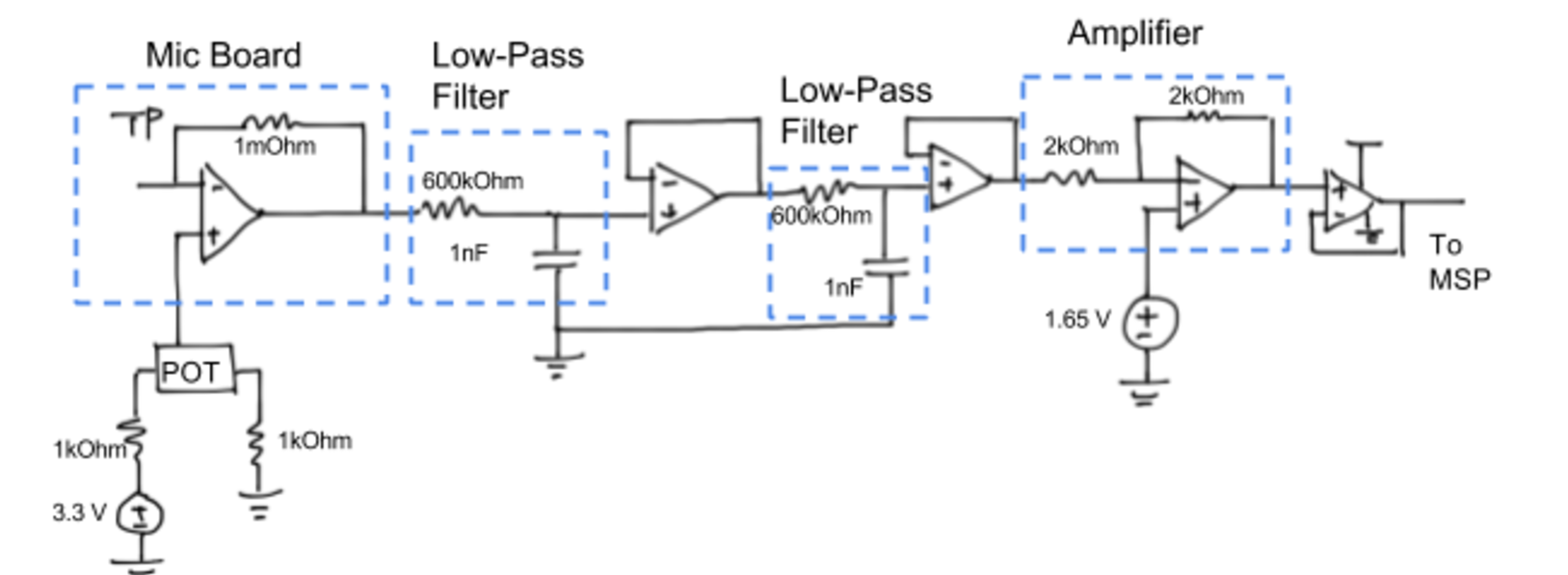
To center the microphone output signal at 1.65 volts, the output of a potentiometer is set at the positive terminal of the op-amp at the end of the mic-circuit. The potentiometer was then tuned until the signal had the correct center frequency. The signal was then passed through two low pass filters to remove aliasing. The transfer function for the two low pass filters was 1(jwRC + 1)2 , which meant that the cutoff frequency was 1RC. To get a cutoff frequency of 1,500 Hz, we used three 200 kresistors in series (600 k total resistance) and a capacitor value of 1 nF. This set the cutoff frequency at 1667 Hz. We had a strong signal so no amplification was necessary. As a result, we used the same resistor values (2 k) across the amplifier circuit. Between each of these circuits, a buffer was added so each circuit does not influence the circuits around them.
|
|
The first component of the front-end circuit is the final op-amp of the mic board, which gives a non-inverting amplification of 2. For the two low pass filters that follow the microphone, the gain as a function of frequency starts at 0, then drops off at a slope of -40 db/decade at the cutoff frequency of 1,500 Hz. The phase starts at 0, then drops off starting at 150 Hz, ending at -180 degrees at 15,000 Hz. Because the two resistors in the non-inverting gain after the low pass filters are the same, there is a gain of 1 at the op-amp. This component is not necessary for our final circuit, but we left the gain there in case we needed to tune the microphone amplification. The signal then enters a buffer (no significant effect on gain or frequency response) before it gets outputted to the micro-controller
We used “accelerate” to instruct the car to move forward quickly, “automatic” to turn the car right, “tic-tac-toe” to turn the car left, and “pipe” to make the car move forward slowly.
Initially, we used the words “race car”, “automatic”, “exhaust”, “pipe”. We later changed “race car” to “accelerate” because the data points for “race car” are overlapping with “exhaust”. We also changed the word “exhaust” to “tic tac toe” because the centroid for “exhaust” is too close to “accelerate”. We chose “tic tac toe” because it has three syllables. These are the steps to performing PCA classification. Step 1: Record and plot the four voice commands. Select a certain time segment so that the four commands don’t look the same (Length: 110). We had the snippet length originally set to 60, but the words “tic-tac-toe” and “pipe” look too similar so we extended it to 110. Step 2: We then stack the four voice commands together into a matrix and run the SVD code on it. When looking at the sigma values of the SVD, it shows that we need two principal components. Step 3: Run K-means Classifications on the different data points and find four centroids, one for each command. These centroids will later serve as reference points. When a new command comes in at run time, it will check which centroid the new input is closest to and classify to that command. Initially when we have the snippet length set to 60, the 3rd and 4th word have centroids that are too close to each other and there is a high chance that the classifier will misclassify. We then change the snippet length to 110 so that longer words were not cut off. To make our classification system more robust, we added a loudness threshold and a K-means threshold to the integration code. If we are not speaking to the microphone, the data the microphone takes in does not need to be analyzed. Therefore, if the peak sound input is not greater than a loudness threshold, the listen mode reruns. If the loudness threshold passes and the word said into the microphone is not clearly matched with one of our four command words, the K-means threshold eliminates the data, meaning no command is passed to the car. This way, the car moves only when we want it to and in the way that we want it to.
|
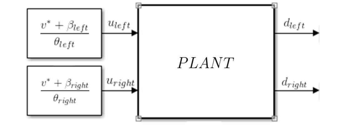
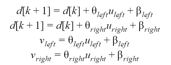
The block diagram in Figure 2 is the open loop model implemented as our first form of control. In this model, v*is the desired speed for the car, and adjusts each input to guess the inputs required to make the car go straight, and PLANT represents the car, which takes in uleftand urightas inputs and outputs data from the photointerrupter sensors of the displacement of each wheel. To find the theta and beta values, we took in dynamics data on the two wheel to see how they react to various inputs. We then used a least squares regression on the following equations to calculate the theta and beta values and therefore find the relationship between the inputs and motor velocities.
|
Using this model of the motor dynamics, we found the following values: left=3.76361507308, right=4.25231985664, left=402.924884735, and right=465.05255718. Using these equations, we can solve for uleft and uright to find each input as a function of desired speed. Now, we can input the same speed for both the left and right motors, and the car should, in theory, drive straight. The implementation of this can be seen in Figure 2 above. Because there is no feedback in this system, the controller uses dead reckoning to guess inputs for making the car go straight.
After running the open loop control system on the car, we noticed the car would still turn to one side even though the car should go straight according to the dynamics data collected. This is because the slight angles in the caster wheel in the rear can constantly push the car to one side, and the same inputs to the motors does not always result in the motors turning at the same speeds. To fix this issue, a closed-loop control system is required so the car can correct itself when it starts straying from driving in a straight line.
|
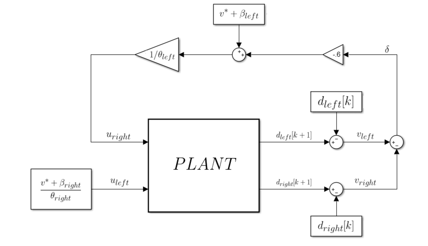
Our final closed loop diagram can be seen in figure 3 above. In this diagram, the beta and theta values had the same values as the open loop control system, and the gain of -.6 in the upper right is the controller gain for the left motor. When we first started working with closed-loop control of the cart, the cart would overcorrect small deviations from driving straight, so we removed the closed-loop control on the right motor and let the left motor correct itself to the speed of the right motor (more details on why we did this is in the following section). We also taped our rear caster wheel because the wheel turns to one side even when the car is trying to drive straight, which sometimes causes the car’s drive wheels to slip on the ground, rendering the car unable to correct its non-forward motion.
Originally we used the two k values found given in the code as closed loop gains. However the cart kept overcorrecting, no matter what k values we gave it (from borderline unstable high values of .7 down to .008). We then used an open loop control for the right motor and had the left motor converge onto the speed of the right motor, which resulted in our robot driving straight. A gain of -.6 was used for optimal performance. Higher values of k (in magnitude) responded to noise in the sensor readings (so the car turned even when it did not have to) and lower values of k (in magnitude) caused the car to respond too slowly to itself turning. To turn, we added constant values to the calculation of delta (the difference in speed between the left wheel and the right wheel) to make the robot think it is turning so it would correct itself (the controller would try to set the delta term to zero, which results in the car turning). For the same constant values, the robot would turn at different rates, so we ended up subtracting 1600 from the delta to turn left and adding 500 to turn right.
A benefit of doing this project is being able to intuitively understand how to apply the concepts learned in class. Lectures and homework problems are good for developing a good theoretical understanding of controls engineering, but working on a project is extremely beneficial for understanding how concepts are applied. Using the project, we learned that simply taking dynamics data and applying inputs based on this data is not enough to make the car go straight (open-loop control). Because a lot of disturbances and noise exist in the real world, a closed-loop control system is necessary to make the car go straight. It was also helpful to learn the basics of artificial intelligence by using K-means to classify words that we say to the robot.