Overview
This project is broken down into two sections:
Section I: Rasterization
\(\quad\) Part 1: Rasterizing single-color triangles
\(\quad\) \(\quad\) Coloring pixels by determining if center point is within a triangle.
\(\quad\) Part 2: Antialiasing triangles
\(\quad\) \(\quad\) Coloring pixels with averaged values.
\(\quad\) Part 3: Transforms
\(\quad\) \(\quad\) Performing transformations on a group of triangles.
Section II: Sampling
\(\quad\) Part 4: Barycentric coordinates
\(\quad\) Part 5: "Pixel sampling" for texture mapping
\(\quad\) Part 6: "Level sampling" with mipmaps for texture mapping
I think it's fair to call this project a journey. From doing simple pixel colorings to performing group transformation and later to map a texture onto a world map. This has definitely changed the way I look at computer generated images. The concept behind supersampling is astonishing. Instead of striving to generate a clear binary cut image all the time, in graphics, you sometimes try to color pixels in intermediate colors in order to preserve the characteristics of an object. I also find the texture mapping of the project mind blowing.Before working on this project, I had thought texture to be something to be coded pixel by pixel. The idea that we can do a simple mapping is both intriguing and powerful.
Section I: Rasterization
Part 1: Rasterizing single-color triangles
Rasterize Triangles: In the process to color each pixel, we check if the middle point of each pixel is within a triangle mesh. Triangles are represented using three indices \(V_A, V_B, V_C\). To check whether a point is within a triangle, you first find the line equations for the three sides \(l_1, l_2, l_3\). Next, find the vectors from each indices to the point. Let's call these vectors \(v_1, v_2, v_3\). As long as \(\langle l_i, v_i \rangle > 0\, \forall i=1,2,3\) or \( \langle l_i, v_i \rangle \leq 0, \forall i=1, 2, 3\), then we can say that the point is in the triangle. Once we know the point is in particular triangle, we color the pixel accordingly.
In order to minimize the number of pixels to check, I only attempt to color the pixels that are inside the triangle. Given points \((x_0, y_0), (x_1, y_1), (x_2, y_2)\), I set the following parameters:
\(x_direction_lower_bound = min(x_0, x_1, x_2)\)
\(x_direction_upper_bound = max(x_0, x_1, x_2)\)
\(y_direction_lower_bound = min(y_0, y_1, y_2)\)
\(y_direction_upper_bound = max(y_0, y_1, y_2)\)
After I found the boundaries, I simply traverse through the pixels row by row, column by column.
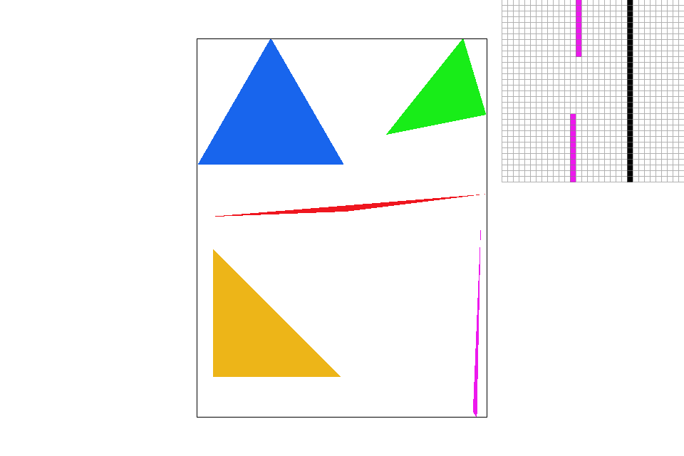
Included below are the results of coloring different triangles and their respective zoomed in screenshots
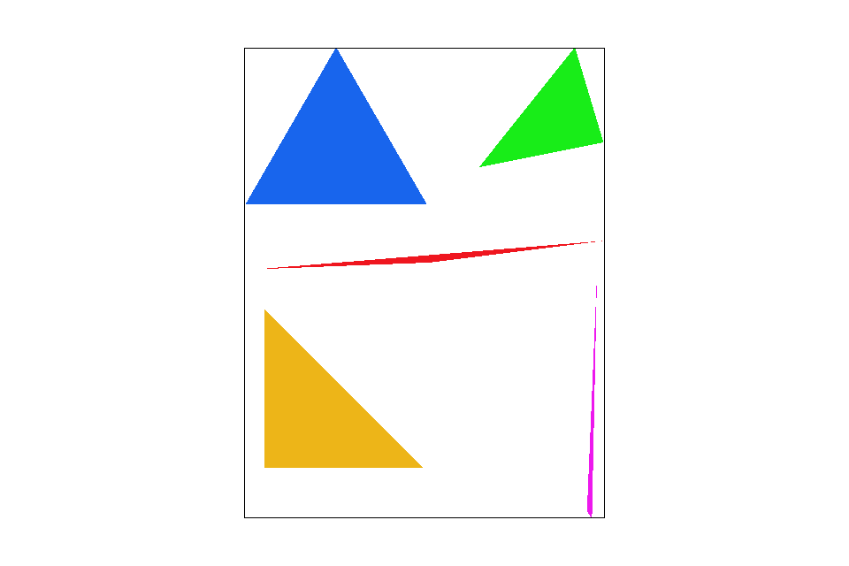
Rasterizing single-color triangles. |
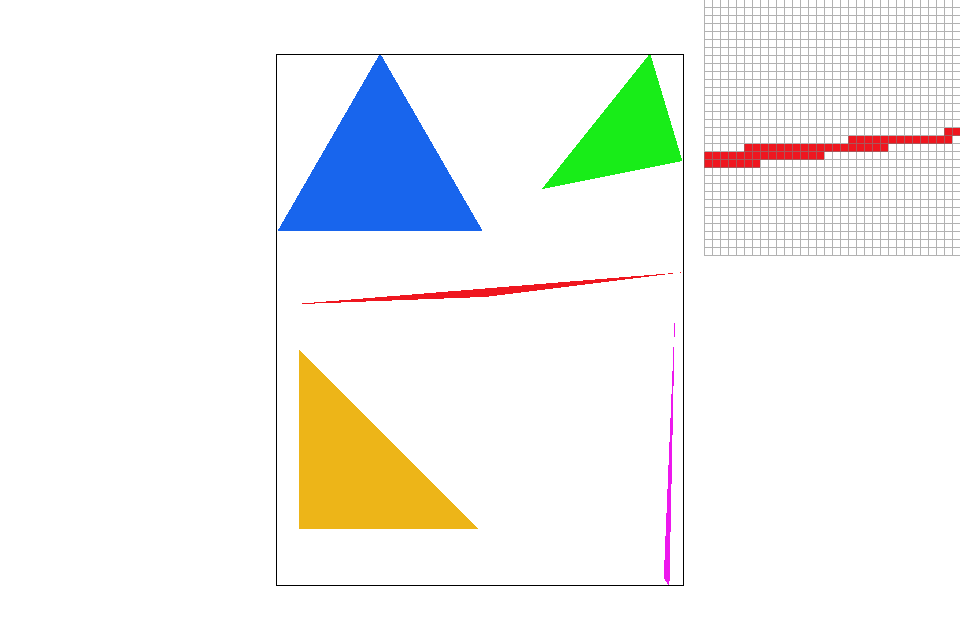
Zooming in on the edge of the red triangle |

Zooming in on the edge of the blue triangle. |

Zooming in on the edge of the purple triangle. |
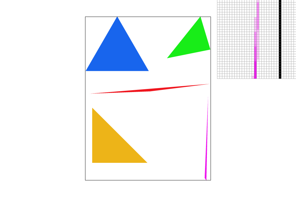
Part 2: Antialiasing triangles
Supersampling takes a pixel and break it down into multiple subpixels, all of which are also squares. This implicitly means that the number of subpixels in each pixel is a perfect square. By averaging the color in all the subpixels in a pixel, we can get an intermediate value between 0 and 1. The last step would be to color that pixel according to the ratio we just calculated.
Modifications made to the rasterization pipeline: Within the for loops of traversing through the pixels, I created additional two for loops to traverse through the subpixels. After filling in the colors for each pixel, using the method mentioned in part 1, I find the average value of the subpixels and assign a color to the pixel accordingly.
Sampling Rate: Number of subpixels within a pixel. (This should be a perfect square number)
Sample Rate 1 |

Sample Rate 4 |

Sample Rate 9 |
Sample Rate 16 |
The effects of supersampling is more obvious when observing the sharp edge of the purple triangle. As the sample rate increases, we can see the edge starts to blur out and eventually connects the broken segments.
Part 3: Transforms
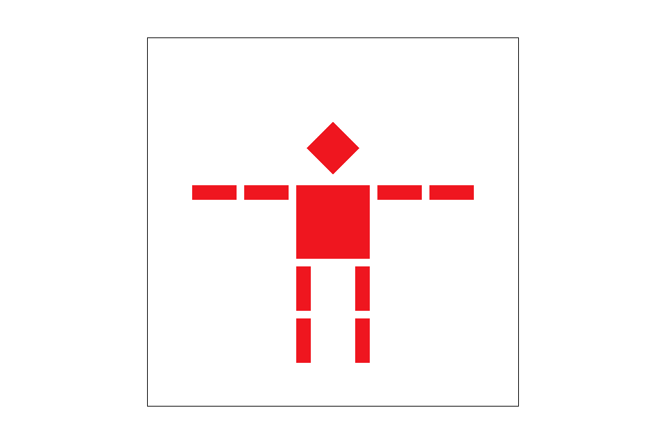
Cube man from project skeleton |
With some translation and rotation, the robot can do some interesting moves!
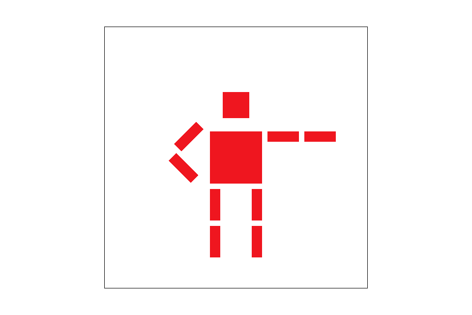
The robot is pointing to the right side of the screen |
Section II: Sampling
Part 4: Barycentric coordinates
Barycentric Coordinates is a tuple of three numbers \(\alpha, \beta, \gamma \) corresponding to the weight placed at the three vertices of a triange. \(V_A, V_B, V_C\). Given the three indices of a triangle \(V_A, V_B, V_C\), we can find values \(\alpha, \beta, \gamma \) that satisfies the following equations. $$V = \alpha V_A + \beta V_B + \gamma V_C$$ $$\alpha + \beta + \gamma = 1$$ $$V: geometric\ centroid $$
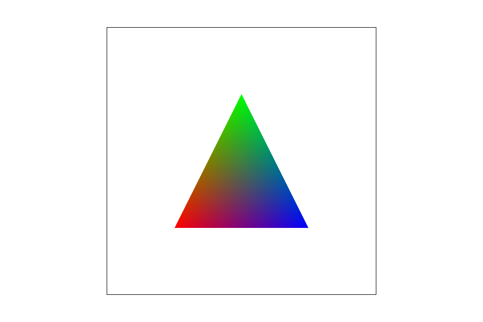
Barycentric coordinates linearly interpolate values at vertices |
svg/basic/test7.svg default viewing parameters and sample rate 1 |
In Figure 4-1. For each point in the triangle, depending on the distance from each point to each vertices, it is asigned a different weight of the "vertices". In this scenario, the vertices represent three different colors (red, green, blue).
Part 5: "Pixel sampling" for texture mapping
Pixel sampling is the process of looking up the position on the texture that each pixel corresponds to. Even if the texture is the same size as the space, positions on the texture might map to complete different positions on the space. Hence, this is where sampling comes into play.
We will be discussing two different pixel sampling methods: Nearest Sampling and Bilinear Sampling
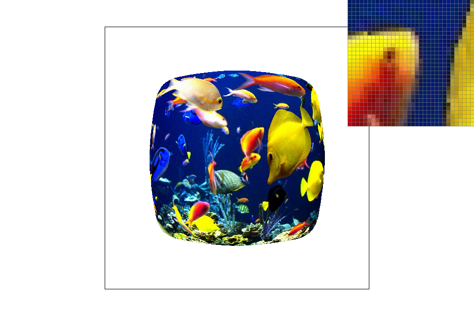
Nearest Sampling: This sampling method uses the color of the texel closest to the pixel center. While it does not require a lot of computation, it results in a "blocky" map. Given a set of coordinates on the texture plane, \((u, v)\), simply convert it to \((x, y)\) coordinates
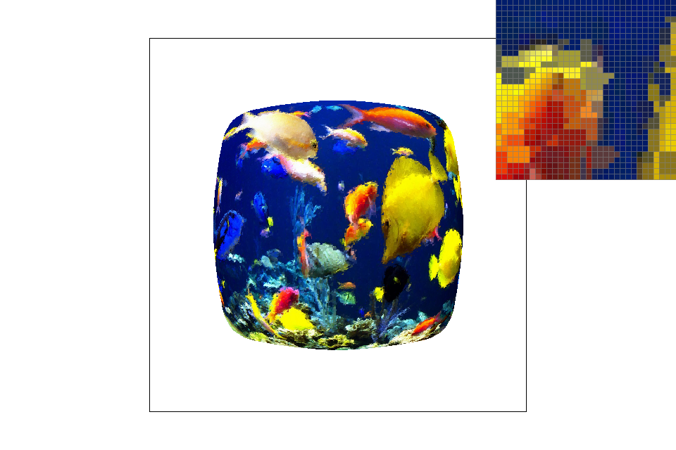
Bilinear Sampling: This sampling method samples the four nearest texels and find the weighted average according to the distance between the point and the four texels. This results in a smoother gradient change compare to Nearest Sampling.
For better contrast, we will be zooming into Italy on the world map.

Nearest Sampling at 1 sample per pixel |

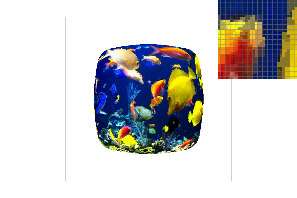
Nearest Sampling at 16 samples per pixel |

Bilinear Sampling at 1 sample per pixel |

Bilinear Sampling at 16 sample per pixel |
If we simply look at images that are sampled at 1 sample per pixel (Figure 5-1 and Figure 5-3), we can see from the zoomed in picture with nearest sampling has more "color jumps" than the one done with bilinear sampling. Images sampled at 16 sample per pixel show an even larger contrast (Figure 5-2 and Figure 5-4).
Part 6: "Level sampling" with mipmaps for texture mapping
In Part 5, we simplified the texture mapping process by only looking at a world space that has the same size as the texture space. In the case of minification and magnification, we will be using mipmaps. We can think of mipmaps as layers of images with each layer representing a lower resolution from the one below it of the same image.
In deciding which Mipmap level to sample from, there are three different sampling methods:
1. Sampling from the zero-th MipMap. (L_ZERO)
2. Sampling from the nearest MipMap level (L_NEAREST)
3. Perform bilinear sampling on the two nearest adjacent MipMap levels and perform trilinear sampling. (L_LINEAR)
Computing Mipmap Level \(D\):
Given \( \frac{du}{dx}, \frac{dv}{dx}, \frac{du}{dy}, \frac{dv}{dy}\), with \(u, v \) as the coordinates in the texture space and \(x, y\) the coordinates in the world space. The MipMap level \(D\) is found from the following equations:
$$L = max(\sqrt{(\frac {du}{dx})^2 + \frac{dv}{dx})^2}, \sqrt{(\frac {du}{dy})^2 + \frac{dv}{dy})^2})$$
$$D = log_2{L}$$
After deciding on the MipMap level, we can then perform either Nearest Sampling or Bilinear Sampling like in Part 5.
1. P_NEAREST: Nearing Sampling
2. P_LINEAR: Bilinear Sampling
| P_NEAREST | P_LINEAR | |
| L_ZERO |
|

|
| L_NEAREST |

|
|
| L_LINEAR |
|

|
From comparing the images, we can see that sampling from the zeroth level has best result. And from sampling the same level, bilinear sampling shows a less "blocky" image. In general, L_LINEAR should take up a larger memory spae than L_ZERO or L_NEAREST. L_ZERO and L_NEAREST should take up approximately the same amount of memory space because it only needs to sample from one mipmap level. In terms of computation time, L_LINEAR \(\geq\) L_NEAREST \(\geq\) L_ZERO.