Assignment 3: PathTracer

Overview: There are 5 parts to this project:

Part 1: Ray Generation and Intersection

Shooting rays from the camera and find the intersection points for triangles and spheres.

Part 2: Bounding Volume Hierarchy

Because testing ray and primitive intersection requires too much computation, we can limit the number of calculation by implementing a Bounding Volume Hierarchy.

Part 3: Direct Illumination

Estimates the direct lighting at a point after ray hits.

Part 4: Indirect Illumniation

Estimates the indirect lighting at a point after ray hits.

Part 5: Adaptive Sampling

The big idea is that we don't usually need to sample uniformly for all pixels because some pixels converge faster than others. We can utilize this property and apply adaptive sampling to lower the number of samples.

Part 1: Ray Generation and Intersection

There are 4 tasks in Part 1.

Task 1: Filling in the sample loop

In PathTracer::raytrace_pixel(size_t x, size_t y), generate camera rays for each pixel. The x and y passed into function are the bottom left corner of the pixel. Depending on the number of samples that we want to smaple, we iterate through num_samples, evaluate the radiance for each sample and sum them up in the end.

Task 2: Generating camera rays

In Camera:generate_ray(), generate rays in the camera space.

Task 3: Intersecting Triangles

In Triangle::intersect(), calculate whether a ray is intersecting with a triangle and initialize the intersection. Each intersection object has 4 attributes that needs to be updated here. Those include t, normal, primitive, and bsdf. t and bsdf are pretty intuitive. The normal attribute is calculated through the barycentric of the normals of the triangles around the current triangle. primitive is used to store the primitive object that the ray is intersecting with, in this case, it is the triangle itself.

Task 4: Intersecting Spheres

In Sphere::intersect(const Ray& r), I calculate the intersection of the ray pased in with the current sphere if there exist an intersection. A helper function Sphere::test() is implemented to test the existence of an intersection. Here, I mainly use b^2-4*a*c to check for a valid intersections (There are three possible cases: no intersection, one intersection, and two intersections).

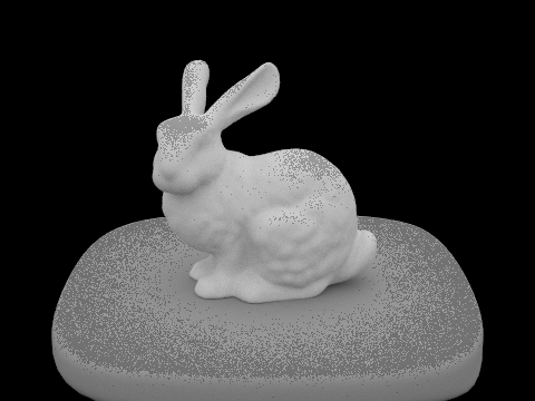
Included in the following are some sipmle dae files. These are files that do not require a BVH structure for it to render faster because the small number of primitives.

Part 2: Bounding Volume Hierarchy

There are 3 tasks for part 2

Task 1: Constructing the BVH

After the implementation from part 1, we are traversing through every single mesh, which is really inefficient when rendering images with lots of meshes. The idea is to create a BVH (Bounding Volume Hierarcy) to decrease the number of meshes that we need to check that intersects with a ray. Initially, I tried to implement the BVH structure according to the dimension of the box, cutting the longest axis in half. However, I realized afterwards that this might not be the best approach because it's possible that all the meshes are crowded at one side of the box.

In the end, I decided to split primitives according to centroids, that way, is is more likely each children of a box has equal numbers of primitives.

The trickest part in implementing this is the edge case when all primitives are classied to the same children, leaving the other children with zero primitives. A termination is needed to make sure that this function doesn't go in a loop.

Task 2: Intersecting BBox

Bbox stands for bounding box. On a fundamental level, we want to be able to calculate the intersection of a ray with a bounding box. This will be used for BVHAccel::intersect() in task 3.

Task 3: Intersecting BVHAccel

After constructing the BVH structure, the next step is to implement BVHAccel::intersect() in order to calculate the intersections of the ray and primitives.

Included in the following are some dae files with greater number of meshes.

Part 3: Direct Illumination

Task 1: Diffuse BSDF

In this project, we are only implementing diffuse BSDF. There are two functions that needed to be implemented: DiffuseBSDF::f and DiffuseBSDF::sample_f

Task 2: Direct lighting

On a higher level, the function estimate_direct_lighting estimates the direct lighting at a point after ray hits. The first step is to traverse through all the light sources in a scene, take samples from the surface of each light, compute the corresponding incoming radiance from those sampled directions, and lastly calculate the outgoing radiance according to the material's BSDF.

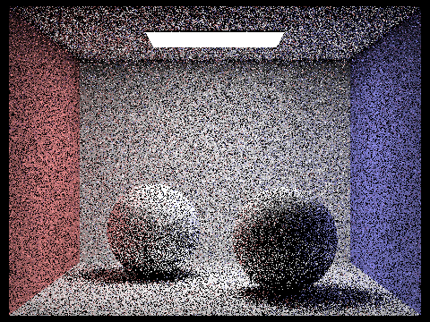
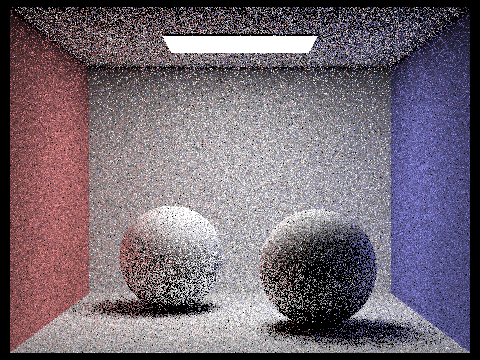
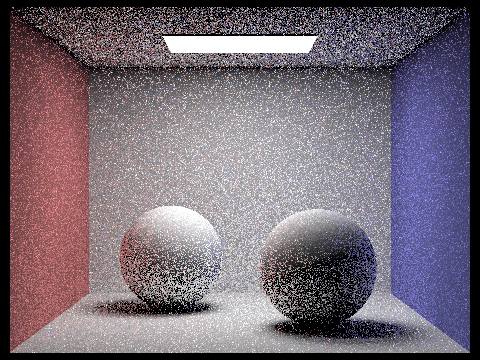
The top surface of the spheres are having less and less noise as the number of light rays goes up. The finaly image still looks like it contains a lot of noise, this is because the image is rendered with 1 sample per pixel.

Part 4: Indirect Illumination

Walk through of implementation of the indirect lighting function

The function estimate_indirect_lighting estimates the indirect lighting at a point after a ray hit. To implement this, I take a sample from the BSDF of the hit point and trace that direction.

Some implementation details: I'm multiplying illum() by 10 and add it a constant 0.05 so that it doesn't terminate too early and result in high noise.

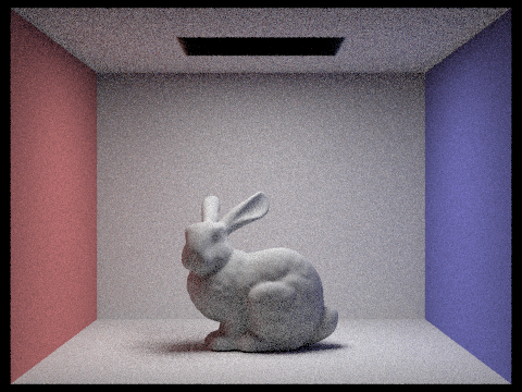
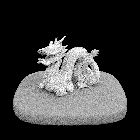
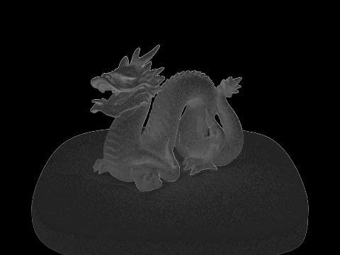
Pick one scene and compare rendered views first with only direct illumination, then only indirect illumination.

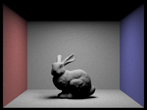
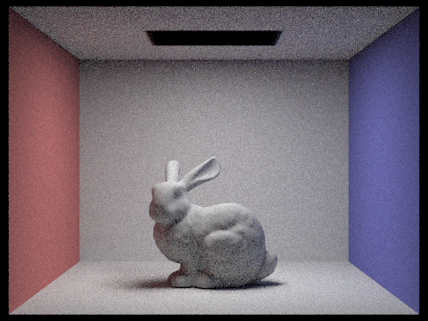
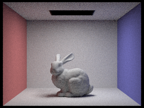
For CBbunny.dae, compare rendered views with max_ray_depth equal to 0, 1,2, 3, and 100 (the -m flag)

max_ray_depth decides the number of light bounces, hence for max_ray_depth = 0, 1, 2, 3, there is an obvious light up of the scene. However, because the energy of each light ray drops with each bounce, there are no obvious difference between images with max_ray_depth=3 and max_ray_depth = 100

Pick one scene and compare rendered views with various sample-per-pixel rates, inluding at least 1, 2, 4, 8, 16, 64, and 1024. Use 4 light rays.

Images with higher sample-per-pixel rate have higher resolutions. In the case of the last image with 1024 sample-per-pixel, I think it's because it was ran with only a small number of lightrays.

Part 5: Adaptive Sampling

Walk through the implementation of the adaptive sampling

The big idea is that we don't usually need to sample uniformly for all pixels, with some pixels converging faster than others.

First, we need find a condition for the pixel to converge and stop tracing more rays. To implement this, I first find the mean mu and standard deviation sigmaof the traced n samples through a pixel, and use this found standard deviation to calculate I. I = 1.96*sigma/sqrt(n). If I <= maxTolerance*mu with maxTolerance = 0.05, then we know that the pixel has already converged and we can stop tracing more rays.

A scene rendered with the maximum numer of samples per pixel at least 2048. 1 sample per light and at least 5 for max ray depth.